Introduction to Computer Vision
Georgia Tech CS 4476 Fall 2019 edition
Project 5: Scene Recognition with Bag of Words
Brief
- Due: 11/18/2019 11:59PM
- Project materials including writeup template proj5_v2.zip
- Data to be used: data.zip: download and extract to the project folder
- Hand-in: through Canvas AND Gradescope
- Required files:
<your_gt_username>.zipon Canvas<your_gt_username>_proj5.pdfon Gradescope
Setup
We will be installing a NEW environment for this project; follow the instructions below to set up the env. If you run into import module errors, try “pip install -e .” again, and if that still doesn’t work, you may have to create a fresh environment.
- Install Miniconda. It doesn’t matter whether you use Python 2 or 3 because we will create our own environment that uses 3 anyway.
- Create a conda environment using the appropriate command. On Windows, open the installed “Conda prompt” to run the command. On MacOS and Linux, you can just use a terminal window to run the command, Modify the command based on your OS (
linux,mac, orwin):conda env create -f proj5_env_<OS>.yml - This should create an environment named ‘proj5’. Activate it using the Windows command,
activate proj5or the MacOS / Linux command,source activate proj5 - Install the project package, by running
pip install -e .inside the repo folder. - Run the notebook using
jupyter notebook ./proj5_code/proj5.ipynb - Ensure that all sanity checks are passing by running
pytesteither inside the “proj5_unit_tests/” folder, or directly in the project directory. - Generate the zip folder for the code portion of your submission once you’ve finished the project using
python zip_submission.py --gt_username <your_gt_username>and submit to Canvas (don’t forget to submit your report to Gradescope!).
Dataset:
The dataset to be used in this assignment is the 15-scene dataset, containing natural images in 15 possible scenarios like bedrooms and coasts. It’s first introduced by Lazebnik et al, 2006. The images have a typical size of around 200 by 200 pixels, and serve as a good milestone for many vision tasks. A sample collection of the images can be found below:
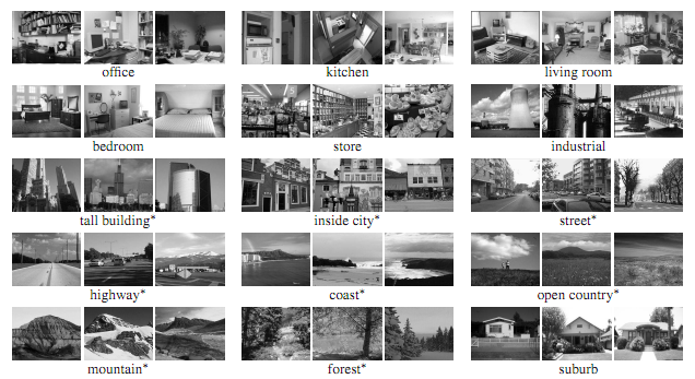
Example scenes from each of the categories of the dataset.
Part 1: Tiny Image Representation and Nearest-neighbor Classification
Learning Objective: (1) Understanding the tiny image representation and (2) set up the workflow for nearest-neighbor classification.
Introduction
We start by implementing the tiny image representation and the nearest neighbor classifier. They are easy to understand, easy to implement, and run very quickly for our experimental setup (less than 10 seconds).
The “tiny image” feature, inspired by the work of the same name by Torralba, Fergus, and Freeman, is one of the simplest possible image representations. One simply resizes each image to a small, fixed resolution (we recommend 16x16). It works slightly better if the tiny image is made to have zero mean and unit length. This is not a particularly good representation, because it discards all of the high frequency image content and is not especially invariant to spatial or brightness shifts. Torralba, Fergus, and Freeman propose several alignment methods to alleviate the latter drawback, but we will not worry about alignment for this project. We are using tiny images simply as a baseline. See get_tiny_images() in the starter code for more details.
The k nearest-neighbors classifier is equally simple to understand. When tasked with classifying a test feature into a particular category, one simply finds the k “nearest” training examples (L2 distance is a sufficient metric; you’ll be implementing this in pairwise_distance()) and assigns the test case the label of the most common neighbor out of the k nearest neighbors. The k nearest neighbor classifier has many desirable features – it requires no training, it can learn arbitrarily complex decision boundaries, and it trivially supports multiclass problems. The voting aspect also alleviates training noise. K nearest neighbor classifiers also suffer as the feature dimensionality increases, because the classifier has no mechanism to learn which dimensions are irrelevant for the decision. The k neighbor computation also becomes slow for high dimensional data and many training examples. See nearest_neighbor_classify() for more details.
Together, the tiny image representation and nearest neighbor classifier will get about 15% to 25% accuracy on the 15 scene database. For comparison, chance performance is ~7%.
Part 1.1: Pairwise Distances
Implement pairwise_distances() in student_code.py. Use the Euclidean distance metric found here: (https://en.wikipedia.org/wiki/Euclidean_distance). You’ll be using your implementation of pairwise_distances() in nearest_neightbor_classify(), kmeans(), kmeans_quantize(). Please note that you are NOT allowed to use any library functions like pairwise_distances from sklearn or pdist from scipy to help you do the calculation.
Part 1.2: Tiny Image Representation
Fill in the function get_tiny_images() to return a Numpy array of dimension \(N \times d\), where \(N\) is the number of image instances and \(d\) is the output feature dimension. In our case, our features are a \(16 \times 16\) tiny image, so the feature dimension \(d\) is a flattened array of length 256.
Part 1.3: K Nearest-Neighbors Classification
In student_code.py, implement the function nearest_neighbor_classify(). Given the training image features and labels, together with the testing features, classify the testing labels using the k nearest neighbors found in the training set. Your k nearest neighbors would vote on what to label the data point. The pipeline in the Jupyter Notebook will also walk you through the performance evaluation via a simple confusion matrix.
Paste the confusion matrix with the standard parameters (image size = 16\(\times\)16, k = 3) onto the report. Note that you need to tune your parameters and reach 15% to get full credits for this part.
Experiment and Report:
Perform experiments with the values of
- tiny image size;
kin kNN.
More specifically, test with the following image sizes: 8\(\times\)8, 16\(\times\)16, 32\(\times\)32, and the following k: 1, 3, 5, 15. Compare the performance against the standard parameter (image size = 16\(\times\)16, k = 3) and report the accuracy. You will see a difference in both processing time and final accuracy; why is that?
Part 2: Bag-of-words with SIFT Features
Learning Objective: (1) Understanding the concept of visual words, (2) set up the workflow for k-means clustering to construct the visual vocabulary, and (3) combine with the previous implemented k nearest-neighbor pipeline for classification.
Introduction
After you have implemented a baseline scene recognition pipeline it is time to move on to a more sophisticated image representation – bags of quantized SIFT features. Before we can represent our training and testing images as a bag of feature histograms, we first need to establish a vocabulary of visual words. We will form this vocabulary by sampling many local features from our training set (10’s or 100’s of thousands) and then clustering them with k-means. The number of k-means clusters is the size of our vocabulary and the size of our features. For example, you might start by clustering many SIFT descriptors into k=50 clusters. This partitions the continuous, 128-dimensional SIFT feature space into 50 regions. For any new SIFT feature we observe, we can figure out which region it belongs to as long as we save the centroids of our original clusters. Those centroids are our visual word vocabulary. Because it can be slow to sample and cluster many local features, the starter code saves the cluster centroids and avoids recomputing them on future runs. See build_vocabulary() for more details.
Now we are ready to represent our training and testing images as histograms of visual words. For each image we will densely sample many SIFT descriptors. Instead of storing hundreds of SIFT descriptors, we simply count how many SIFT descriptors fall into each cluster in our visual word vocabulary. This is done by finding the nearest k-means centroid for every SIFT feature. Thus, if we have a vocabulary of 50 visual words, and we detect 220 SIFT features in an image, our bag of SIFT representation will be a histogram of 50 dimensions where each bin counts how many times a SIFT descriptor was assigned to that cluster and sums to 220. A more intuitive way to think about this is through the original bag-of-words model in NLP: assume we have a vocab of [“Messi”, “Obama”], and article A contains 15 occurrences of “Messi” with 1 “Obama”, while article B with 2 “Messi” and 10 “Obama”, then we may safely assume that article A is focusing on sports and B on politics, relatively speaking (unless Messi actually decides to run for the president).
The histogram should be normalized so that image size does not dramatically change the bag of feature magnitude. See get_bags_of_sifts() for more details.
You should now measure how well your bag of SIFT representation works when paired with a k nearest-neighbor classifier. There are many design decisions and free parameters for the bag of SIFT representation (number of clusters, sampling density, sampling scales, SIFT parameters, etc.) so accuracy might vary from 40% to 60%.
Part 2.1: k-means
In student_code.py, implement the function kmeans() and kmeans_quantize(). Note that in this part you are NOT allowed to use any clustering function from scipy or sklearn to perform the k-means algorithm. Here kmeans() is used to perform the k-means algorithm and generate the centroids given the raw data points; kmeans_quantize() will assign the closest centroid to each of the new data entry by returning the indices. For the max_iter parameter, the default value is 100, but you may start with small value like 10 to examine the correctness of your code; 10 is also sufficiently good to get you a decent result coupling with proper choice of k in kNN.
Part 2.2: Build the Visual Vocab
In student_code.py, implement the function build_vocabulary(). For each of the training images, sample SIFT features uniformly: for this part, start from the pixel location (10, 10) on the image, and retrieve the SIFT feature with a stride size of 20 for both horizontal and vertical directions. Concatenate all features from all images, and perform k-means on this collection; the resulting centroids will be the visual vocabulary. We have provided a working edition of SIFTNet for you to use in this part.
Part 2.3: Put it together with kNN Classification
Now that we have obtained a set of visual vocabulary, we are now ready to quantize the input SIFT features into a bag of words for classification. In student_code.py, implement the function get_bags_of_sift(), and complete the classification workflow in the Jupyter Notebook. Sample uniformly from both training and testing images for their SIFT features (you may want to sample with a smaller stride size), and quantize the features according to the vocab we’ve built (which centroid should be assigned to the current feature?), and by computing the vocab histogram of all the features for a particular image, we are able to tell what’s the most important “aspect” of the image. Given both “aspects” for training and testing images, since we know the ground truth for the training features, we can use nearest-neighbor to identify the labels for the testing feature.
Again, in this part, you need to tune your parameters and obtain a final accuracy of at least 45% to get full credits for this part.
Experiment and Report:
You may want to play around with different values for the following parameters:
vocab_size: start from 50, and you may choose to go up to 200max_iterinkmeans(): 10 will be sufficiently good to get at least 40% accuracystrideorstep_sizein bothbuild_vocabulary()andget_bags_of_sifts()kin kNN
As the processing time for this section could be dangerously long, we don’t impose a fixed list of values to try here. Instead, paste the confusion matrix with your best result onto the report, and record your param settings.
Similarly, during the experiments you must have witnessed the difference when you are tuning the params. Specifically, when you fix all other parameters and apply kNN, experiment with k value and report the performance difference. Compare the difference here versus the k value experiment in Part 1: what can you tell from it?
Extra Credits
Performance:
- up to 2 pts: without using any additional classifier, reach a final accuracy of 60%;
- Hints: you may need to change your kNN using different distance metrics.
Model:
- up to 5 pts: set up the experiment with SVM, and reach the accuracy of 65%;
- Hints: you may take a look at the
SVCclassifier insklearn; also note that common case of SVC classifies object following the one-against-one scheme, so you may need to do some extra work to make it fit in the multi-class problem. If you manage to get an accuracy above 60%, add that to your report!
- Hints: you may take a look at the
Writeup
For this project (and all other projects), you must do a project report using the template slides provided to you. Do not change the order of the slides or remove any slides, as this will affect the grading process on Gradescope and you will be deducted points. In the report you will describe your algorithm and any decisions you made to write your algorithm a particular way. Then you will show and discuss the results of your algorithm. The template slides provide guidance for what you should include in your report. A good writeup doesn’t just show results–it tries to draw some conclusions from the experiments. You must convert the slide deck into a PDF for your submission.
If you choose to do anything extra, add slides after the slides given in the template deck to describe your implementation, results, and analysis. Adding slides in between the report template will cause issues with Gradescope, and you will be deducted points. You will not receive full credit for your extra credit implementations if they are not described adequately in your writeup.
Rubric
- +70 pts: Code
- 30 pts: Part 1
- 40 pts: Part 2
- +30 pts: PDF report
- 15 pts: Part 1
- 15 pts: Part 2
- -5*n pts: Lose 5 points for every time you do not follow the instructions for the hand-in format.
Submission Format
This is very important as you will lose 5 points for every time you do not follow the instructions. You will have two submission files for this project:
<your_gt_username>_proj5.zipvia Canvas containing:proj5_py/- directory containing all your code for this assignment
<your_gt_username>_proj5.pdfvia Gradescope - your report
Do not install any additional packages inside the conda environment. The TAs will use the same environment as defined in the config files we provide you, so anything that’s not in there by default will probably cause your code to break during grading. Do not use absolute paths in your code or your code will break. Use relative paths like the starter code already does. Failure to follow any of these instructions will lead to point deductions. Create the zip file using python zip_submission.py --gt_username <your_gt_username> (it will zip up the appropriate directories/files for you!) and hand it through Canvas. Remember to submit your report as a PDF to Gradescope as well.
Credit
Assignment developed by Shenhao Jiang, Jacob Knaup, Julia Chen, Stefan Stojanov, Frank Dellaert, and James Hays based on a similar project by Aaron Bobick.