Introduction to Computer Vision
Georgia Tech CS 4476 Fall 2019 edition
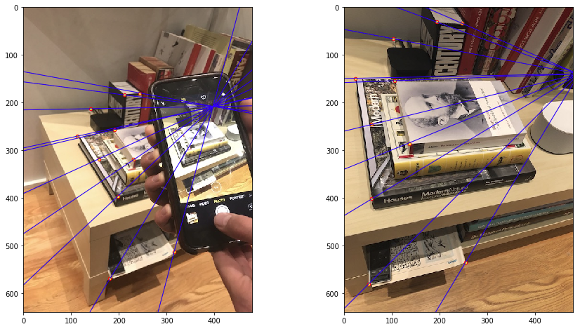
Epipolar lines showing camera locations given corresponding points in two views of a scene.
Project 3: Camera Projection Matrix and Fundamental Matrix Estimation with RANSAC
Brief
- Due:
- 10/16/2019 11:59PM
- Project materials including writeup template proj3_v3.zip
- Hand-in: through Canvas AND Gradescope
- Required files:
<your_gt_username>.zipon Canvas<your_gt_username>_proj3.pdfon Gradescope
Setup
Note that we will be using a new environment for this project! If you run into import module errors, try “pip install -e .” again, and if that still doesn’t work, you may have to create a fresh environment.
- Install Miniconda. It doesn’t matter whether you use Python 2 or 3 because we will create our own environment that uses 3 anyways.
- Create a conda environment using the appropriate command. On Windows, open the installed “Conda prompt” to run the command. On MacOS and Linux, you can just use a terminal window to run the command, Modify the command based on your OS (
linux,mac, orwin):conda env create -f proj3_env_<OS>.yml - This should create an environment named ‘proj3’. Activate it using the Windows command,
activate proj3or the MacOS / Linux command,source activate proj3 - Install the project package, by running
pip install -e .inside the repo folder. - Run the notebook using
jupyter notebook ./proj3_code/proj3.ipynb - Ensure that all sanity checks are passing by running
pytestinside the “unit_tests/” folder. - Generate the zip folder for the code portion of your submission once you’ve finished the project using
python zip_submission.py --gt_username <your_gt_username>and submit to Canvas (don’t forget to submit your report to Gradescope!).
Part 1: Camera Projection Matrix Estimation
Learning Objective: (1) Understanding the the camera projection matrix and (2) estimating it using fiducial objects for camera projection matrix estimation and pose estimation.
Introduction
In this first part you will perform pose estimation in an image taken by an uncalibrated camera. As we saw in class, pose estimation is incredibly useful; it is used in VR, AR, controller tracking, autonomous driving, and even satellite docking. Recall that for a pinhole camera model, the camera matrix \(P \in \mathbb{R}^{3\times4}\) is a projective mapping from world (3D) to pixel (2D) coordinates defined up to a scale.
\[\begin{align} \mathbf{x} = f(\mathbf{X}_w;\mathbf{P}) = \mathbf{P}\mathbf{X}_w = \begin{bmatrix} u \\ v \\ 1 \end{bmatrix} \cong \begin{bmatrix} s \cdot u \\ s \cdot v \\ s \end{bmatrix} = \begin{bmatrix} p_{11} & p_{12} & p_{13} & p_{14} \\ p_{21} & p_{22} & p_{23} & p_{24} \\ p_{31} & p_{32} & p_{33} & p_{34} \\ \end{bmatrix} \begin{bmatrix} x_w \\ y_w \\ z_w \\ 1 \end{bmatrix}. \end{align}\]Above \(s\) is an arbitrary scale factor. The camera matrix can also be decomposed into intrinsic parameters \(\mathbf{K}\) and extrinsic parameters \(\mathbf{R}^T\left[\mathbf{I}\mid -\mathbf{t} \right]\).
\[\mathbf{P} = \mathbf{K}\mathbf{R}^T[\mathbf{I}\;|\; -\mathbf{t}].\] \[\mathbf {P}= \begin{bmatrix} \alpha & s & u_0 \\ 0 & \beta & v_0 \\ 0 & 0 & 1 \end{bmatrix} \begin{bmatrix} r_{11} & r_{21} & r_{31} \\ r_{12} & r_{22} & r_{32} \\ r_{13} & r_{23} & r_{33} \end{bmatrix} \begin{bmatrix} 1 & 0 & 0 & -t_x \\ 0 & 1 & 0 & -t_y \\ 0 & 0 & 1 & -t_z \end{bmatrix}\]Let’s look more carefully into what each of the individual parts of the decomposed matrix mean. The homogenous vector coordinates \((x_w, y_w, z_w,1)\) of \(\mathbf{X}_w\) indicate the position of a point in 3D space in the world coordinate system. The matrix \([\mathbf{I}\;\mid\; -\mathbf{t}]\) represents a translation and the matrix \(\mathbf{R}^T\) represents a rotation. When combined they convert points from the world to the camera coordinate system. An intuitive way to understand this is to think about how aligning the axes of the world coordinate system to the ones of the camera coordinate system can be done with a rotation and a translation.
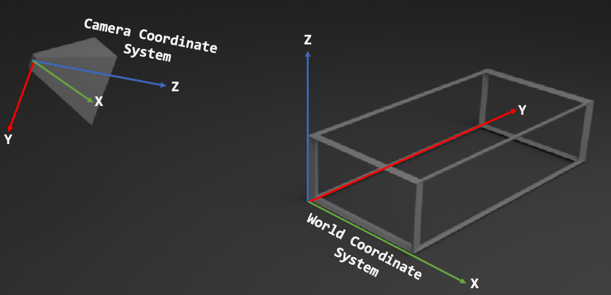
The distinction between camera coordinate and world coordinate systems is a rotation and a translation.
In this part of the project you will learn how to estimate the projection matrix using objective function minimization, how you can decompose the camera matrix, and what knowing these lets you do.
Part 1.1: Implement Camera Projection
In projection_matrix.py you will implement camera projection in the projection(P, points_3d) from homogenous world coordinates \(X_i = [X_i, Y_i, Z_i, 1]\) to non-homogenous image coordinates \(x_i, y_i\).
Given the projection matrix \(\mathbf{P}\), the equation that accomplish this are:
\[\begin{align} x_i = \frac{p_{11}X_i+p_{12}Y_i + p_{13}Z_i + p_{14}}{p_{31}X_i+p_{32}Y_i + p_{33}Z_i + p_{34}} \quad y_i = \frac{p_{21}X_i+p_{22}Y_i + p_{23}Z_i + p_{24}}{p_{31}X_i+p_{32}Y_i + p_{33}Z_i + p_{34}}. \end{align}\]Part 1.2: Implement Objective Function
A camera projection matrix maps points from 3D into 2D. How can we use this to estimate its parameters? Assume that we have \(N\) known 2D-3D correspondences for a set of points, that is, for points with index \(i= 1\dots N\) we have both access to the respective 3D coordinates \(\mathbf{x}_w^{i}\) and 2D coordinates \(\mathbf{x}^{i}\). Let \(\hat{\mathbf{P}}\) be an estimation for the camera projection matrix. We can determine how accurate the estimation is by measuring the reprojection error
\[\sum_{i=1}^N (\hat{\mathbf{P}}\mathbf{x}_w^i-\mathbf{x}^i )^2\]between the 3D points projected into 2D \(\hat{\mathbf{P}}\mathbf{x}_w^i\) and the known 2D points \(\mathbf{x}^i\), both in non-homogenous coordinates. Therefore we can estimate the projection matrix itself by minimizing the reprojection error with respect to the projection matrix
\[\underset{\hat{\mathbf{P}}}{\arg\min}\sum_{i=1}^N (\hat{\mathbf{P}}\mathbf{x}_w^i-\mathbf{x}^i )^2 .\]In this part, in projection_matrix.py you will implement the objective function objective_function() that will be passed to scipy.optimize.least_squares for minimization with the Levenberg-Marquardt algorithm.
Part 1.3: Estimating the Projection Matrix Given Point Correspondences
Optimizing the reprojection loss using Levenberg-Marquardt requires a good initial estimate for \(\mathbf{P}\). This can be done by having good initial estimates for \(\mathbf{K}\) and \(\mathbf{R}^T\) and \(\mathbf{t}\) which you can multiply to then generate your estimated \(\mathbf{K}\). In this part, to make sure that you have the least squares optimization working properly we will provide you with an initial estimate. In the function you will have to implement in this part, estimate_projection_matrix(), you will have to pass the initial guess to scipy.optimize.least_squares and get the appropriate output.
Note: because \(P\) has only 11 degrees of freedom, we fix \(\mathbf{P}_{34=1}\).
Part 1.4: Decomposing the Projection Matrix
Recall that \(\mathbf{P} =\mathbf{K}{}_w\mathbf{R}^T_c[\mathbf{I}\;|\; -{}_w\mathbf{t}_c]\). Rewriting this gives us:
\[\mathbf{P} =[\mathbf{K}{}_w\mathbf{R}^T_c\;|\; \mathbf{K}{}_w\mathbf{R}^T_c -{}_w\mathbf{t}_c] = [\mathbf{K}{}_c\mathbf{R}_w\;|\; \mathbf{K}{}_c\mathbf{t}_w] = [\mathbf{M}\;|\; \mathbf{K}{}_c\mathbf{t}_w].\]Where \(\mathbf{M} = \mathbf{K}{}_c\mathbf{R}_w\) is the first 3 columns of \(\mathbf{P}\). An operation known as RQ decomposition which will decompose \(\mathbf{M}\) into an upper triangular matrix \(\mathbf{R}\) and an orthonormal matrix \(\mathbf{Q}\) such that \(\mathbf{RQ} = \mathbf{M}\), where the upper triangular matrix will correspond to \(\mathbf{K}\) and the ortonormal matrix to \({}_c\mathbf{R}_w\). In this part you will implement decompose_camera_matrix(P) where you will need to get the appropriate matrix elements of \(\mathbf{P}\) to perform the RQ decomposition, and make the appropriate function call to scipy.linalg.rq().
Part 1.5: Calculating the Camera Center
In this part in projection_matrix.py you will implement calculate_camera_center(P, K, R) that takes as input the
projection \(\mathbf{P}\), intrinsic \(\mathbf{K}\) and rotation \({}_c\mathbf{R}_w\) matrix and outputs the camera position in world coordinates.
Part 1.6: Taking Your Own Images and Estimating the Projection Matrix + Camera Pose
In part 1.3 you were given a set of known points in world coordinates. In this part of the assignment you will learn how to use a fiducial—an object of known size that can be used as a reference. Any object for which you have measured the size given some unit (in this project you should use centimeters).
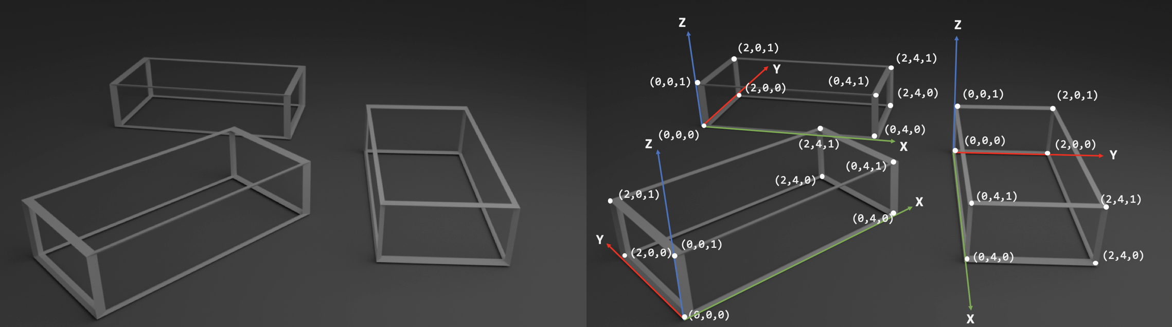
Example of how one cuboid of known dimensions can be used as a fiducial to create multiple world coordinate systems
The figure above illustrates how a cuboid of known dimension can be used to create a world coordinate system and a set of points with known 3D location. Choose an object that you will use as a fiducial (we recommend using a thick textbook) and measure it. Using a camera capture two images of the object (you will estimate the camera parameters for both images) keeping in mind the considerations discussed in class for part 2 and fundamental matrix estimation if you want to reuse these images. When taking the images, try to estimate the pose of the camera lens of your phone in the world coordinate system.
Now that you have the dimension of your object (3D points), you can use the Jupyter notebook to find the image coordinates of the 3D points create your own 2D-3D correspondences for each image. For each of your 2 images, make initial estimates for \(\mathbf{P}\) and if your estimate is good, using your code from the previous part you should be able to estimate both the the projection matrix and the camera pose. Use the code available in the Jupyter notebook to visualize your findings.
Report
Put these answers in your report!
- What would happen to the projected points if you increased/decreased the \(x\) coordinate, or the other coordinates of the camera center \(\mathbf{t}\)? Write down a description of your expectations in the appropriate part of your writeup submission.
- Perform this shift for each of the camera coordinates and then recompose the projection matrix and visualize the result in your Jupyter notebook. Was the visualized result what you expected?
Part 2: Fundamental Matrix Estimation
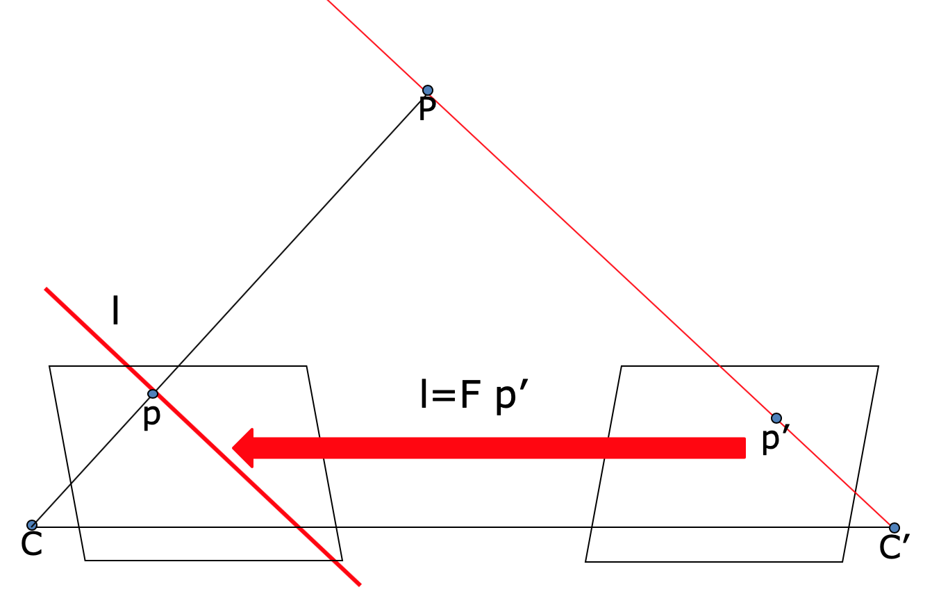
Diagram of epipolar lines and epipoles. The fundamental matrix maps points from one image to an epipolar line on the other.
Learning Objective: (1) Understanding the fundamental matrix and (2) estimating it using self-captured images to estimate your own fundamental matrix.
In this part, given a set of corresponding 2D points, we will estimate the fundamental matrix. Now that we know how to project a point from a 3D coordinate to a 2D coordinate, next we’ll look at how to map corresponding 2D points from two images of the same scene. You can think of the fundamental matrix as something that maps points from one view into a line in the other view. We get a line because a point in one image is only a projection to 2D, which means we can’t actually know the “depth” of that point. As such, from the viewpoint of the other camera, we can see the entire “line” that our first point could exist on.
The fundamental matrix constraint between two points \(x_0\) and \(x_1\) in the left and right views, respectively, is given by the following equation:
\[x_0^TFx_1=0\]Above \(x_0\) and \(x_1\) are homogenous coordinates in the two views, and \(F\) is the \(3 \times 3\) fundamental matrix. We can write out the equation above as:
\[\begin{bmatrix} u_0 & v_0 & 1 \end{bmatrix} \begin{bmatrix} f_{11} & f_{12} & f_{13}\\ f_{21} & f_{22} & f_{23}\\ f_{31} & f_{32} & f_{33}\\ \end{bmatrix} \begin{bmatrix} u_1\\ v_1\\ 1 \end{bmatrix} =0\]Since \(F\) takes points in one image and maps them to a line in another image, the constraint says that we want the point \(x_0\) to be on the line represented by \(Fx_1\). If the point is exactly on the line, then the constraint \(x^T_1Fx_1=0\) and the line-to-point distance between them is also zero.
Hence to estimate \(F\) we can minimize the line-to-point distance between the point \(x_0\) and the line \(Fx_1\), for all matching points \((x_0, x_1)\). This makes estimating the fundamental matrix a least squares problem.
Part 2.1: Distance Formula
The line-to-point distance formula \(d\) is defined by the following equation:
\[d(l, x) = \frac{au + bv + c}{\sqrt{a^2 + b^2}}\]where \(1 = [a,b,c]\) is a line and \(x = [u, v, 1]\) is the homogenous coordinate for the point. You will need to implement this in point_line_distance() in fundamental_matrix.py.
Part 2.2: Symmetric line-to-point error
Given a set of matching points \(\{x_0^i, x_1^i\}\) we can set up the following symmetric line-to-point error function for every match \((x_0,x_1)\).
\[d(Fx_1, x_0)^2 + d(F^T x_0, x_1)^2\]where \(d\) is the distance formula between a line and a point, \(x_0\) is one of the homogeneous points, \(F\) is the fundamental matrix, and \(x_1\) is the other homogeneous point. In the first term we use \(F\), which maps from the second to the first view, and in second term we use \(F^T\), which maps from the first to the second view. SciPy handles the squaring and summing for you so you just need to implement point_line_distance().
By applying this symmetric line-to-point error calculation to every pair of points, we get this equation for the objective function to minimize, as a function of \(F\):
\[J(F) = \sum_i^n \bigg( d(Fx_1^i, x_0^i)^2 + d(F^T x_0^i, x_1^i)^2 \bigg)\]This is the equation you will be implementing in signed_point_line_errors() which is in the file fundamental_matrix.py.
Part 2.3: Least Squares Optimization
Since this is a least squares optimization problem, you will also be making the call to SciPy’s least squares optimizer. The documentation for this is available here. You’ll need to give as input: the objective function, your initial estimate of the fundamental matrix, optimization algorithm, method for computing the Jacobian, and the point pairs. There are more details on this in the code.
Part 2.4: Try it Yourself
Similar to Part 1, you’ll have to take two images of the same scene and estimate the fundamental matrix between the two images. Recall that these two images must be from different positions, and you cannot simply just rotate the camera or zoom the image. You’ll have to save the images in the same project folder and use the Jupyter notebook to run your fundamental matrix estimator on your images.
Report
Put these answers in your report!
- Why is it that when you take your own images, you can’t just rotate the camera or zoom the image for your two images of the same scene?
- Why is it that points in one image are projected by the fundamental matrix onto epipolar lines in the other image?
- What happens to the epipoles and epipolar lines when you take two images where the camera centers are within the images? Why?
- What does it mean when your epipolar lines are all horizontal across the two images?
- Why is the fundamental matrix defined up to a scale?
- Why is the fundamental matrix rank 2?
Part 3: RANSAC
Now you have a function which can calculate the fundamental matrix \(F\) from matching pairs of points in two different images. However, having to manually extract the matching points is undesirable. In the previous project, we implemented SIFTNet to automate the process of identifying matching points in two images. Below is a high-level description of how we will implement this section. See the Jupyter notebook and code documentation for implementation details.
We will implement a pipeline to run two images through SIFTNet to extract matching points and then send those points to your fundamental matrix estimation function to acheive an automated process for generating the fundamental matrix \(F\). However, there is an issue with this. Previously, the manually-identified points were perfect matches between your two images. As we saw before, SIFT does not generate matches with 100% accuracy. Fortunately, to calculate the fundamental matrix \(F\), we need only 9 matching points and SIFT can generate hundreds, so there should be more than enough good matches somewhere in there (if only we can find them).
We will use a method called RANdom SAmple Consensus (RANSAC) to search through the points returned by SIFT and find true matches to use for calculating the fundamental matrix \(F\). Please review the lecture slides on RANSAC to refresh your memory on how this algorithm works. Additionally, you can find a simple explanation of RANSAC at https://www.mathworks.com/discovery/ransac.html. See section 6.1.4 in the textbook for a more thorough explanation of how RANSAC works.
In summary, we will implement a workflow using the SIFTNet from project 2 to extract feature points, then RANSAC will select a random subset of those points, you will call your function from Part 2 to calculate the fundamental matrix \(F\) for those points, and check how many other points identified by SIFTNet match \(F\). Then you will iterate through this process until you find the subset of points that produces the best fundamental matrix \(F\) with the most matching points.
Report
Put these answers in your report!
- How many RANSAC iterations would we need to find the fundamental matrix with 99.9% certainty from your Mount Rushmore and Notre Dame SIFTNet results assuming that they had a 90% point correspondence accuracy?
- One might imagine that if we had more than 9 point correspondences, it would be better to use more of them to solve for the fundamental matrix. Investigate this by finding the number of RANSAC iterations you would need to run with 18 points.
- If our dataset had a lower point correspondence accuracy, say 70%, what is the minimum number of iterations needed to find the fundamental matrix with 99.9% certainty?
At the end of this assignment you will be performing RANSAC to find the fundamental matrix for an image pair that you create, and you will want to keep the estimated accuracy of your point correspondences in mind when deciding how many iterations are appropriate.
Testing
We have provided a set of tests for you to evaluate your implementation. We have included tests inside proj3.ipynb so you can check your progress as you implement each section. When you’re done with the entire project, you can call additional tests by running pytest inside the “./unit_tests” directory of the project. Your grade on the coding portion of the project will be further evaluated with a set of tests not provided to you.
Bells & Whistles (Extra Points)
Reflect on the fundamental matrix and RANSAC songs for extra credit. See the report template for details. Fundamental Matrix Song RANSAC Song
Writeup
For this project (and all other projects), you must do a project report using the template slides provided to you. Do not change the order of the slides or remove any slides, as this will affect the grading process on Gradescope and you will be deducted points. In the report you will describe your algorithm and any decisions you made to write your algorithm a particular way. Then you will show and discuss the results of your algorithm. The template slides provide guidance for what you should include in your report. A good writeup doesn’t just show results–it tries to draw some conclusions from the experiments. You must convert the slide deck into a PDF for your submission.
If you choose to do anything extra, add slides after the slides given in the template deck to describe your implementation, results, and analysis. Adding slides in between the report template will cause issues with Gradescope, and you will be deducted points. You will not receive full credit for your extra credit implementations if they are not described adequately in your writeup.
Rubric
- +66 pts: Code
- 22 pts: Part 1
- 22 pts: Part 2
- 22 pts: Part 3
- +34 pts: PDF report
- 10 pts: Part 1
- 10 pts: Part 2
- 10 pts: Part 3
- 4 pts: Conclusions and tests screenshot
- -5*n pts: Lose 5 points for every time you do not follow the instructions for the hand-in format.
Submission Format
This is very important as you will lose 5 points for every time you do not follow the instructions. You will have two submission files for this project:
<your_gt_username>_proj3.zipvia Canvas containing:proj3_py/- directory containing all your code for this assignment
<your_gt_username>_proj3.pdfvia Gradescope - your report
Do not install any additional packages inside the conda environment. The TAs will use the same environment as defined in the config files we provide you, so anything that’s not in there by default will probably cause your code to break during grading. Do not use absolute paths in your code or your code will break. Use relative paths like the starter code already does. Failure to follow any of these instructions will lead to point deductions. Create the zip file using python zip_submission.py --gt_username <your_gt_username> (it will zip up the appropriate directories/files for you!) and hand it through Canvas. Remember to submit your report as a PDF to Gradescope as well.
Credit
Assignment developed by Jacob Knaup, Julia Chen, Stefan Stojanov, Frank Dellaert, and James Hays based on a similar project by Aaron Bobick.